Motivation

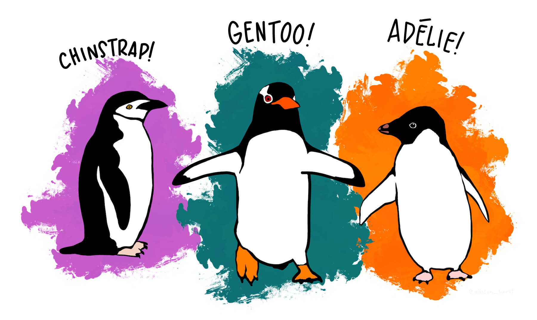
Throughout this section we will be analyzing a dataset about penguins. The name of the dataset is palmerpenguins, which is available as a CRAN package.

To install the palmerpenguins data set

install.packages("palmerpenguins")

Loading data into R

library(palmerpenguins)

Meet the `penguins` data frame or “tibble”

By loading the palmerpenguins package, we now have access to a data frame called penguins. Get an overview of this with str(), which displays the structure of an object.

str(penguins)

tibble [344 × 8] (S3: tbl_df/tbl/data.frame)
 $ species          : Factor w/ 3 levels "Adelie","Chinstrap",..: 1 1 1 1 1 1 1 1 1 1 ...
 $ island           : Factor w/ 3 levels "Biscoe","Dream",..: 3 3 3 3 3 3 3 3 3 3 ...
 $ bill_length_mm   : num [1:344] 39.1 39.5 40.3 NA 36.7 39.3 38.9 39.2 34.1 42 ...
 $ bill_depth_mm    : num [1:344] 18.7 17.4 18 NA 19.3 20.6 17.8 19.6 18.1 20.2 ...
 $ flipper_length_mm: int [1:344] 181 186 195 NA 193 190 181 195 193 190 ...
 $ body_mass_g      : int [1:344] 3750 3800 3250 NA 3450 3650 3625 4675 3475 4250 ...
 $ sex              : Factor w/ 2 levels "female","male": 2 1 1 NA 1 2 1 2 NA NA ...
 $ year             : int [1:344] 2007 2007 2007 2007 2007 2007 2007 2007 2007 2007 ...

str() will provide a sensible description of almost anything and, worst case, nothing bad can actually happen. When in doubt, just str() some of the recently created objects to get some ideas a bout what to do next.

We could print the penguins object itself to screen. However, if you have used R before, you might be reluctant to do this, because large datasets just fill up your console and provide very little insight.

This is the first big win for tibbles. The tidyverse offers a special case of R’s default data frame: the “tibble”, which is a nod to the actual class of these objects, tbl_df.

Now we can boldly print penguins to screen! It is a tibble (and also a regular data frame) and the tidyverse provides a nice print method that shows the most important stuff and doesn’t fill up your Console.

## see? it's still a regular data frame, but also a tibble
class(penguins)

[1] "tbl_df"     "tbl"        "data.frame"

penguins

# A tibble: 344 × 8
   species island    bill_length_mm bill_depth_mm flipper_length_mm body_mass_g
   <fct>   <fct>              <dbl>         <dbl>             <int>       <int>
 1 Adelie  Torgersen           39.1          18.7               181        3750
 2 Adelie  Torgersen           39.5          17.4               186        3800
 3 Adelie  Torgersen           40.3          18                 195        3250
 4 Adelie  Torgersen           NA            NA                  NA          NA
 5 Adelie  Torgersen           36.7          19.3               193        3450
 6 Adelie  Torgersen           39.3          20.6               190        3650
 7 Adelie  Torgersen           38.9          17.8               181        3625
 8 Adelie  Torgersen           39.2          19.6               195        4675
 9 Adelie  Torgersen           34.1          18.1               193        3475
10 Adelie  Torgersen           42            20.2               190        4250
# ℹ 334 more rows
# ℹ 2 more variables: sex <fct>, year <int>

If you are dealing with plain vanilla data frames, you can rein in data frame printing explicitly with head() and tail(). Or turn it into a tibble with as_tibble()!

head(penguins)

# A tibble: 6 × 8
  species island    bill_length_mm bill_depth_mm flipper_length_mm body_mass_g
  <fct>   <fct>              <dbl>         <dbl>             <int>       <int>
1 Adelie  Torgersen           39.1          18.7               181        3750
2 Adelie  Torgersen           39.5          17.4               186        3800
3 Adelie  Torgersen           40.3          18                 195        3250
4 Adelie  Torgersen           NA            NA                  NA          NA
5 Adelie  Torgersen           36.7          19.3               193        3450
6 Adelie  Torgersen           39.3          20.6               190        3650
# ℹ 2 more variables: sex <fct>, year <int>

tail(penguins)

# A tibble: 6 × 8
  species   island bill_length_mm bill_depth_mm flipper_length_mm body_mass_g
  <fct>     <fct>           <dbl>         <dbl>             <int>       <int>
1 Chinstrap Dream            45.7          17                 195        3650
2 Chinstrap Dream            55.8          19.8               207        4000
3 Chinstrap Dream            43.5          18.1               202        3400
4 Chinstrap Dream            49.6          18.2               193        3775
5 Chinstrap Dream            50.8          19                 210        4100
6 Chinstrap Dream            50.2          18.7               198        3775
# ℹ 2 more variables: sex <fct>, year <int>

More ways to query basic info on a data frame:

names(penguins)

[1] "species"           "island"            "bill_length_mm"   
[4] "bill_depth_mm"     "flipper_length_mm" "body_mass_g"      
[7] "sex"               "year"

ncol(penguins)

[1] 8

length(penguins)

[1] 8

dim(penguins)

[1] 344   8

nrow(penguins)

[1] 344

A statistical overview can be obtained with summary()

summary(penguins)

      species          island    bill_length_mm  bill_depth_mm  
 Adelie   :152   Biscoe   :168   Min.   :32.10   Min.   :13.10  
 Chinstrap: 68   Dream    :124   1st Qu.:39.23   1st Qu.:15.60  
 Gentoo   :124   Torgersen: 52   Median :44.45   Median :17.30  
                                 Mean   :43.92   Mean   :17.15  
                                 3rd Qu.:48.50   3rd Qu.:18.70  
                                 Max.   :59.60   Max.   :21.50  
                                 NA's   :2       NA's   :2      
 flipper_length_mm  body_mass_g       sex           year     
 Min.   :172.0     Min.   :2700   female:165   Min.   :2007  
 1st Qu.:190.0     1st Qu.:3550   male  :168   1st Qu.:2007  
 Median :197.0     Median :4050   NA's  : 11   Median :2008  
 Mean   :200.9     Mean   :4202                Mean   :2008  
 3rd Qu.:213.0     3rd Qu.:4750                3rd Qu.:2009  
 Max.   :231.0     Max.   :6300                Max.   :2009  
 NA's   :2         NA's   :2

Bill dimensions

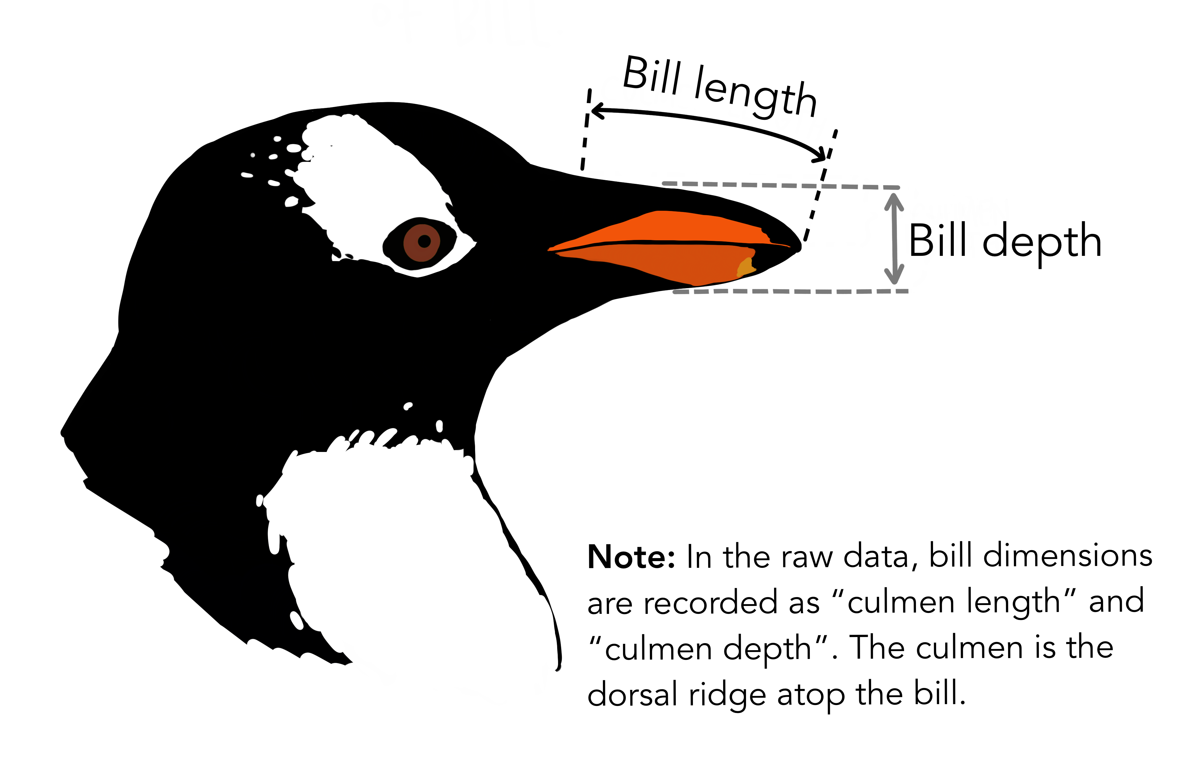
The culmen is the upper ridge of a bird’s bill. In the simplified penguins data, culmen length and depth are renamed as variables bill_length_mm and bill_depth_mm to be more intuitive.

For this penguin data, the culmen (bill) length and depth are measured as shown below

Although we have not begun our formal coverage of visualization yet, it’s so important for data exploration dataset that we will make a few figures anyway. Here we use only base R graphics, which are very basic.

plot(bill_length_mm ~ flipper_length_mm, penguins)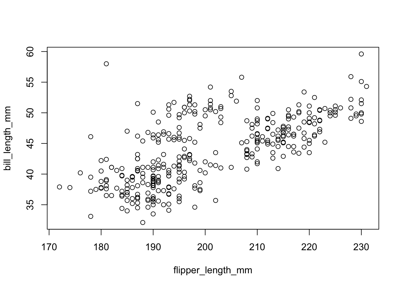

plot(bill_depth_mm ~ bill_length_mm, penguins)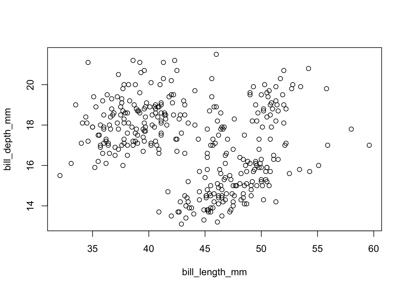

Welcome to the “Tidyverse”

The tidyverse is “an opinionated collection of R packages designed for data science. All packages share an underlying philosophy and common APIs.”

Another way of putting it is that it’s a set of packages that are useful specifically for data manipulation, exploration and visualization with a common philosphy.

What is this common philosphy?

The common philosphy is called “tidy” data. It is a standard way of mapping the meaning of a dataset to its structure.

In tidy data:

Each variable forms a column.
Each observation forms a row.
Each type of observational unit forms a table.

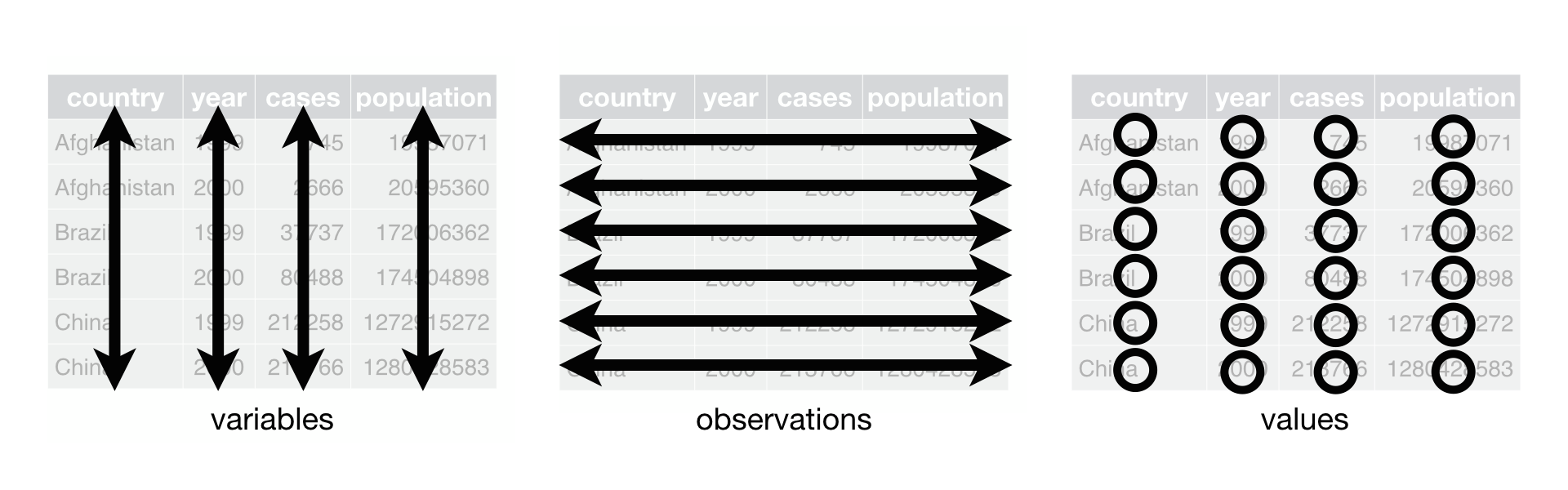
Below, we are interested in transformating the table on the right to the the table on the left, which is considered “tidy”.

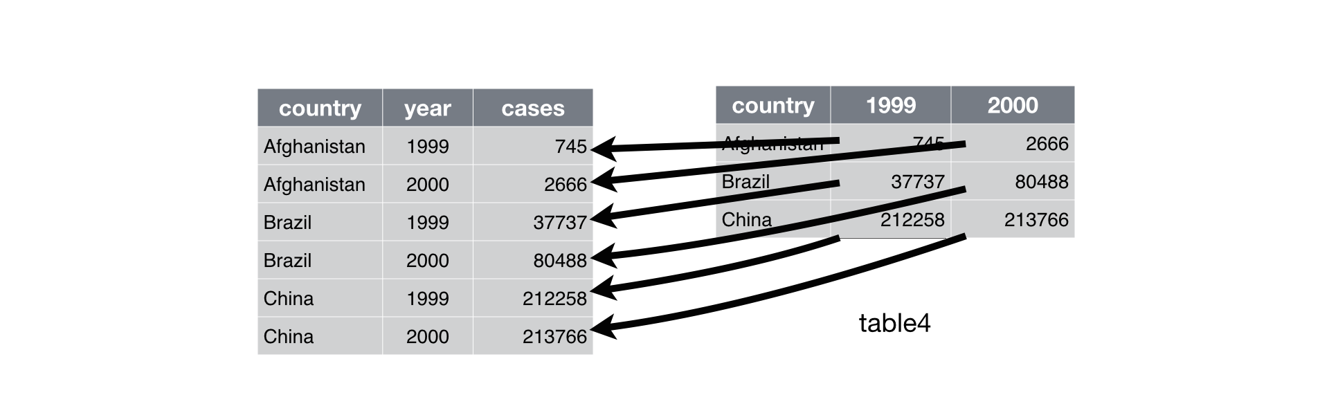
Working with tidy data is useful because it creates a structured way of organizing data values within a data set. This makes the data analysis process more efficient and simplifies the development of data analysis tools that work together. In this way, you can focus on the problem you are investigating, rather than the uninteresting logistics of data.

What is in the `tidyverse`?

We can install and load the set of R packages using install.packages("tidyverse") function.

When we load the tidyverse package using library(tidyverse), there are six core R packages that load:

readr, for data import.
tidyr, for data tidying.
dplyr, for data wrangling.
ggplot2, for data visualisation.
purrr, for functional programming.
tibble, for tibbles, a modern re-imagining of data frames.

Here, we load in the tidyverse.

library(tidyverse)

Because these packages all share the “tidy” philosophy, the data analysis workflow is easier as you move from package to package.

Today we will focus on dplyr and ggplot2, for data wrangling and visualization, but definitely check out the other packages such as readr, tidyr, R packages to import data, to transform data to the “tidy” format.

Data wrangling

In the real world, analyzing data rarely involves data that can be easily imported and ready for analysis. According to Wikipedia:

Data munging or data wrangling is loosely the process of manually converting or mapping data from one “raw” form into another format that allows for more convenient consumption of the data with the help of semi-automated tools.

As you will see in class, one of the most time-consuming aspects of the data analysis process is “data wrangling”. This is also is a trendy term for cleaning up a messy data set.

R provides incredibly powerful and flexible language for data wrangling. However, the syntax is somewhat hard to get used to. We will therefore introducing a package that makes the syntax much more like the English language. This package is dplyr.

The `dplyr` R package

dplyr is a powerful R-package to transform and summarize tabular data with rows and columns.

The package contains a set of functions (or “verbs”) to perform common data manipulation operations such as filtering for rows, selecting specific columns, re-ordering rows, adding new columns and summarizing data.

In addition, dplyr contains a useful function to perform another common task which is the is the “split-apply-combine” concept. We will discuss that in a little bit.

How does it compare to using base functions R?

If you are familiar with R, you are probably familiar with base R functions such as split(), subset(), apply(), sapply(), lapply(), tapply() and aggregate(). Compared to base functions in R, the functions in dplyr are easier to work with, are more consistent in the syntax and are targeted for data analysis around data frames instead of just vectors.

The important dplyr verbs to remember are:

`dplyr` verbs	Description
`select()`	select columns
`filter()`	filter rows
`arrange()`	re-order or arrange rows
`mutate()`	create new columns
`summarize()`	summarize values
`group_by()`	allows for group operations in the “split-apply-combine” concept

Pipe operator: |>

Before we go any futher, let’s introduce the pipe operator: |>.

This operator available in base R allows you to pipe the output from one function to the input of another function. Instead of nesting functions (reading from the inside to the outside), the idea of of piping is to read the functions from left to right.

`dplyr` verbs in action

The two most basic functions are select() and filter() which selects columns and filters rows, respectively.

Selecting columns using `select()`

To select two columns (species and island),

penguins |> 
  select(species, island)

# A tibble: 344 × 2
   species island   
   <fct>   <fct>    
 1 Adelie  Torgersen
 2 Adelie  Torgersen
 3 Adelie  Torgersen
 4 Adelie  Torgersen
 5 Adelie  Torgersen
 6 Adelie  Torgersen
 7 Adelie  Torgersen
 8 Adelie  Torgersen
 9 Adelie  Torgersen
10 Adelie  Torgersen
# ℹ 334 more rows

To select all the columns except a specific column, use the “-” (subtraction) operator (also known as negative indexing).

penguins |> 
    select(-species, -island)

# A tibble: 344 × 6
   bill_length_mm bill_depth_mm flipper_length_mm body_mass_g sex     year
            <dbl>         <dbl>             <int>       <int> <fct>  <int>
 1           39.1          18.7               181        3750 male    2007
 2           39.5          17.4               186        3800 female  2007
 3           40.3          18                 195        3250 female  2007
 4           NA            NA                  NA          NA <NA>    2007
 5           36.7          19.3               193        3450 female  2007
 6           39.3          20.6               190        3650 male    2007
 7           38.9          17.8               181        3625 female  2007
 8           39.2          19.6               195        4675 male    2007
 9           34.1          18.1               193        3475 <NA>    2007
10           42            20.2               190        4250 <NA>    2007
# ℹ 334 more rows

The function select() is much more powerful though. To select a range of columns by name, use the “:” (colon) operator

penguins |> 
  select(bill_length_mm:body_mass_g)

# A tibble: 344 × 4
   bill_length_mm bill_depth_mm flipper_length_mm body_mass_g
            <dbl>         <dbl>             <int>       <int>
 1           39.1          18.7               181        3750
 2           39.5          17.4               186        3800
 3           40.3          18                 195        3250
 4           NA            NA                  NA          NA
 5           36.7          19.3               193        3450
 6           39.3          20.6               190        3650
 7           38.9          17.8               181        3625
 8           39.2          19.6               195        4675
 9           34.1          18.1               193        3475
10           42            20.2               190        4250
# ℹ 334 more rows

To select all columns that end with the character string “c”, use the function ends_with()

penguins |> 
  select(ends_with("mm"))

# A tibble: 344 × 3
   bill_length_mm bill_depth_mm flipper_length_mm
            <dbl>         <dbl>             <int>
 1           39.1          18.7               181
 2           39.5          17.4               186
 3           40.3          18                 195
 4           NA            NA                  NA
 5           36.7          19.3               193
 6           39.3          20.6               190
 7           38.9          17.8               181
 8           39.2          19.6               195
 9           34.1          18.1               193
10           42            20.2               190
# ℹ 334 more rows

Some additional options to select columns based on a specific criteria include

starts_with() = Select columns that start with a character string
contains() = Select columns that contain a character string
matches() = Select columns that match a regular expression
one_of() = Select columns names that are from a group of names

Selecting rows using `filter()`

Let’s say we only want the data from a specific species.

To do this, we can use the filter() function to filter the rows for the Adelie species.

penguins |> 
  filter(species == "Adelie")

# A tibble: 152 × 8
   species island    bill_length_mm bill_depth_mm flipper_length_mm body_mass_g
   <fct>   <fct>              <dbl>         <dbl>             <int>       <int>
 1 Adelie  Torgersen           39.1          18.7               181        3750
 2 Adelie  Torgersen           39.5          17.4               186        3800
 3 Adelie  Torgersen           40.3          18                 195        3250
 4 Adelie  Torgersen           NA            NA                  NA          NA
 5 Adelie  Torgersen           36.7          19.3               193        3450
 6 Adelie  Torgersen           39.3          20.6               190        3650
 7 Adelie  Torgersen           38.9          17.8               181        3625
 8 Adelie  Torgersen           39.2          19.6               195        4675
 9 Adelie  Torgersen           34.1          18.1               193        3475
10 Adelie  Torgersen           42            20.2               190        4250
# ℹ 142 more rows
# ℹ 2 more variables: sex <fct>, year <int>

Note: you can use the boolean operators (e.g. >, <, >=, <=, !=, %in%) to create logical tests.

For example, if we wanted only species with a bill length of greater than or equal to 40, we can add a second criteria:

penguins |> 
  filter(species == "Adelie") |> 
  filter(bill_length_mm >= 40)

# A tibble: 51 × 8
   species island    bill_length_mm bill_depth_mm flipper_length_mm body_mass_g
   <fct>   <fct>              <dbl>         <dbl>             <int>       <int>
 1 Adelie  Torgersen           40.3          18                 195        3250
 2 Adelie  Torgersen           42            20.2               190        4250
 3 Adelie  Torgersen           41.1          17.6               182        3200
 4 Adelie  Torgersen           42.5          20.7               197        4500
 5 Adelie  Torgersen           46            21.5               194        4200
 6 Adelie  Biscoe              40.6          18.6               183        3550
 7 Adelie  Biscoe              40.5          17.9               187        3200
 8 Adelie  Biscoe              40.5          18.9               180        3950
 9 Adelie  Dream               40.9          18.9               184        3900
10 Adelie  Dream               42.2          18.5               180        3550
# ℹ 41 more rows
# ℹ 2 more variables: sex <fct>, year <int>

Use `mutate()` to add new variables

mutate() is a function that defines and inserts new variables into a tibble. You can refer to existing variables by name.

penguins |> 
  mutate(new_ratio = body_mass_g / bill_length_mm) |> 
  select(species, island, new_ratio)

# A tibble: 344 × 3
   species island    new_ratio
   <fct>   <fct>         <dbl>
 1 Adelie  Torgersen      95.9
 2 Adelie  Torgersen      96.2
 3 Adelie  Torgersen      80.6
 4 Adelie  Torgersen      NA  
 5 Adelie  Torgersen      94.0
 6 Adelie  Torgersen      92.9
 7 Adelie  Torgersen      93.2
 8 Adelie  Torgersen     119. 
 9 Adelie  Torgersen     102. 
10 Adelie  Torgersen     101. 
# ℹ 334 more rows

Arrange or re-order rows using `arrange()`

To arrange (or re-order) rows by a particular column such as the bill length, list the name of the column you want to arrange the rows by

penguins |> 
  arrange(bill_length_mm)

# A tibble: 344 × 8
   species island    bill_length_mm bill_depth_mm flipper_length_mm body_mass_g
   <fct>   <fct>              <dbl>         <dbl>             <int>       <int>
 1 Adelie  Dream               32.1          15.5               188        3050
 2 Adelie  Dream               33.1          16.1               178        2900
 3 Adelie  Torgersen           33.5          19                 190        3600
 4 Adelie  Dream               34            17.1               185        3400
 5 Adelie  Torgersen           34.1          18.1               193        3475
 6 Adelie  Torgersen           34.4          18.4               184        3325
 7 Adelie  Biscoe              34.5          18.1               187        2900
 8 Adelie  Torgersen           34.6          21.1               198        4400
 9 Adelie  Torgersen           34.6          17.2               189        3200
10 Adelie  Biscoe              35            17.9               190        3450
# ℹ 334 more rows
# ℹ 2 more variables: sex <fct>, year <int>

If we wanted to arrange in a descending order, we could use the desc() function inside of arrange() to order rows in a descending order.

penguins |> 
  arrange(desc(bill_length_mm))

# A tibble: 344 × 8
   species   island bill_length_mm bill_depth_mm flipper_length_mm body_mass_g
   <fct>     <fct>           <dbl>         <dbl>             <int>       <int>
 1 Gentoo    Biscoe           59.6          17                 230        6050
 2 Chinstrap Dream            58            17.8               181        3700
 3 Gentoo    Biscoe           55.9          17                 228        5600
 4 Chinstrap Dream            55.8          19.8               207        4000
 5 Gentoo    Biscoe           55.1          16                 230        5850
 6 Gentoo    Biscoe           54.3          15.7               231        5650
 7 Chinstrap Dream            54.2          20.8               201        4300
 8 Chinstrap Dream            53.5          19.9               205        4500
 9 Gentoo    Biscoe           53.4          15.8               219        5500
10 Chinstrap Dream            52.8          20                 205        4550
# ℹ 334 more rows
# ℹ 2 more variables: sex <fct>, year <int>

Data visualization

ggplot2

ggplot2 is a powerful data exploration and visualization package that can create graphics in R. It was created by Hadley Wickham when he was a graduate student at Iowa State University and is based on the principals defined in the Grammar of Graphics.

Why is it useful?

The idea of the Grammar of Graphics is to break the graph into components and handle the components of a graph separately. The ggplot2 package contains a set of functions that allow us to build the features of the graph in a series of layers for versatility and control.

There are two main plotting functions in ggplot2:

qplot() = a quick plot, similar to the plot() function in base R
ggplot() = a “grammar of graphics” (gg) plot which is made up two components (a ggplot() object and at least one geom layer)

The ggplot2 is loaded whenever you load tidyverse, but you can always load it formally.

library(ggplot2)

Flipper and bill length

Let’s make a scatter plot of the flipper and bill length for each penguin. We will first make a quick plot of these two variables.

`qplot`

The qplot function allows us to produce simple plots, similar to plot in base R. The main input of qplot is an x and y argument, but it also accepts a data set (data) where the x and y variables are located.

Note

Why does this not work?

qplot(x = flipper_length_mm, y = bill_length_mm)

We need to specify where to get these values from. Instead, we can use the vectors of penguins directly

## need to specify where variables are located
qplot(x = penguins$flipper_length_mm, y = penguins$bill_length_mm)

Warning: `qplot()` was deprecated in ggplot2 3.4.0.

Warning: Removed 2 rows containing missing values (`geom_point()`).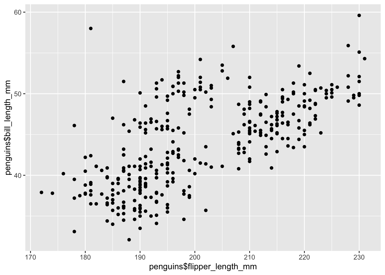

However, a cleaner way to do this is to use the data argument:

qplot(x = flipper_length_mm, y = bill_length_mm, data = penguins)

Warning: Removed 2 rows containing missing values (`geom_point()`).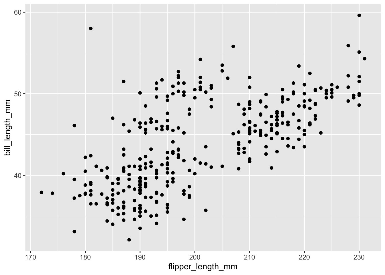

If youw ant to add labels to the x and y axis, you can use the xlab and ylab arguments. You can read the help file to check out other arguments available in the function.

qplot(x = flipper_length_mm, y = bill_length_mm, 
      data = penguins,
      xlab = "Flipper length (mm)", 
      ylab = "Bill length (mm)", 
      main = "Data from palmerpenguins R package")

Warning: Removed 2 rows containing missing values (`geom_point()`).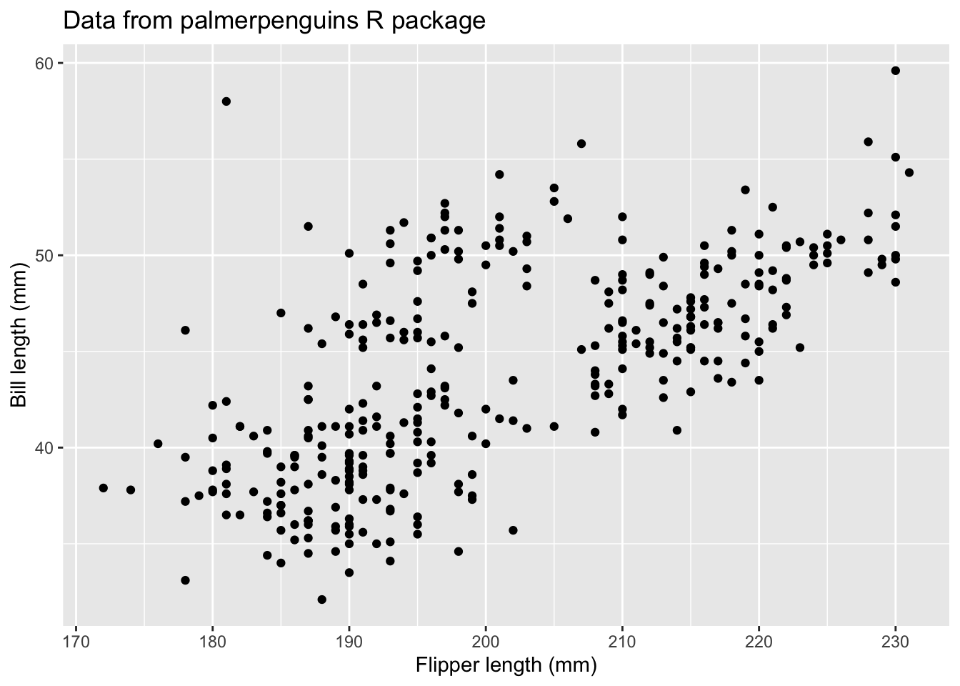

From this plot, we see that there is a positive relationship between the two variables. However, there seems to groups of penguins. Next, we will learn how to color the points using something called the grammar of graphics and create
a series of visualizations.

The `ggplot()` function

This function is the implementation of the “Grammar of Graphics” that allows us to build layers of graphical elements to produce plots. As explained by Hadley Wickham

the grammar tells us that a statistical graphic is a mapping from data to aesthetic attributes (colour, shape, size) of geometric objects (points, lines, bars). The plot may also contain statistical transformations of the data and is drawn on a specific coordinates system.

Terminology

ggplot - the main function where you specify the data set and variables to plot (this is where we define the x and y variable names)
geoms - geometric objects
- e.g. geom_point(), geom_bar(), geom_line(), geom_histogram()
aes - aesthetics
- shape, transparency, color, fill, linetype
scales - define how your data will be plotted
- continuous, discrete, log, etc

There are three ways to initialize a ggplot() object.

An empty ggplot object

ggplot()

A ggplot object associated with a dataset

penguins |> 
  ggplot()

or a ggplot object with a dataset and x and y defined

penguins |> 
  ggplot(aes(x = flipper_length_mm, y = bill_length_mm))

Creating your first ggplot()

We just used the function aes() which is an aesthetic mapping function inside the ggplot() object. We use this function to specify plot attributes (e.g. x and y variable names) that will not change as we add more layers.

Anything that goes in the ggplot() object becomes a global setting. From there, we use the geom objects to add more layers to the base ggplot() object. These will define what we are interested in illustrating using the data.

Earlier we noticed that there was a positive trend between flipper and bill length, but there seemed to be groups of points. Let’s examine this plot with a geom called geom_poin() which is the default when you provide both a x and y variable in the aes() function and add color:

penguins |> 
  ggplot(aes(x = flipper_length_mm, y = bill_length_mm)) + 
  geom_point(aes(color = species))

Warning: Removed 2 rows containing missing values (`geom_point()`).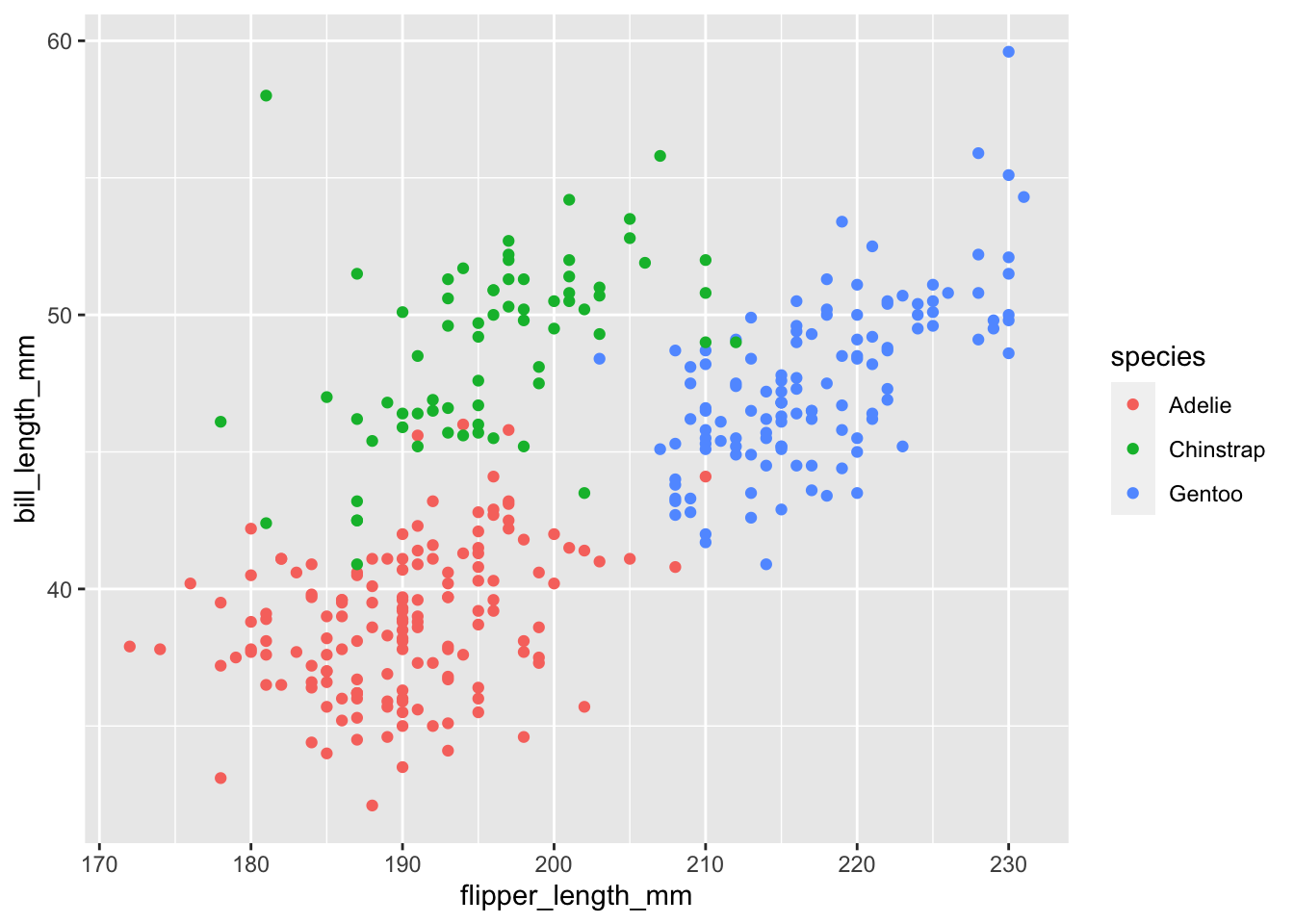

Now we see there groups of points are different species of penguins.

We can also do cool things like there where we add a linear regression line over each species of penguin to see the relationship between the two variables.

penguins |> 
  ggplot(aes(x = flipper_length_mm, 
             y = bill_length_mm, 
             group = species)) + 
  geom_point(aes(color = species)) + 
  geom_smooth(method = "lm", se = FALSE, aes(color = species))

`geom_smooth()` using formula = 'y ~ x'

Warning: Removed 2 rows containing non-finite values (`stat_smooth()`).

Warning: Removed 2 rows containing missing values (`geom_point()`).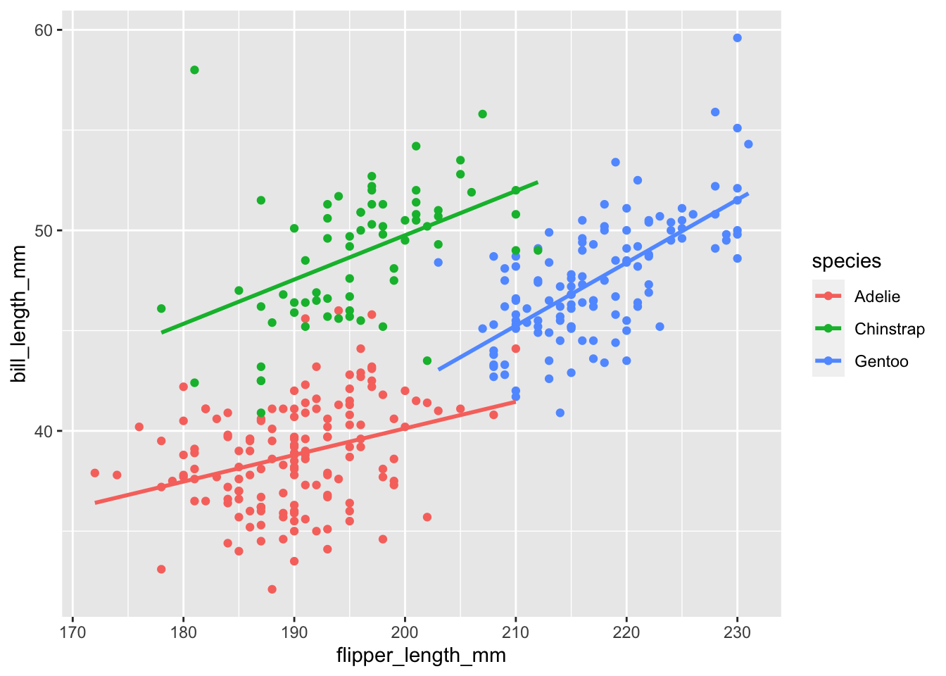

We hope you enjoyed learning about the Tidyverse, data wrangling, and data visualization using a dataset about penguins!

Motivation

Loading data into R

Meet the penguins data frame or “tibble”

Welcome to the “Tidyverse”

What is this common philosphy?

What is in the tidyverse?

Data wrangling

The dplyr R package

How does it compare to using base functions R?

Pipe operator: |>

dplyr verbs in action

Selecting columns using select()

Selecting rows using filter()

Use mutate() to add new variables

Arrange or re-order rows using arrange()

Data visualization

ggplot2

Why is it useful?

Flipper and bill length

qplot

The ggplot() function

Terminology

Creating your first ggplot()

Meet the `penguins` data frame or “tibble”

What is in the `tidyverse`?

The `dplyr` R package

`dplyr` verbs in action

Selecting columns using `select()`

Selecting rows using `filter()`

Use `mutate()` to add new variables

Arrange or re-order rows using `arrange()`

`qplot`

The `ggplot()` function